Modelling Contagion Networks
using Topological Data Analysis and Riemannian Manifolds

Inferring networks from data | Analyzing attributed graphs
Varying degrees of isolation are being put into effect in order to contain the COVID-19 pandemic. These range from simply recommending ‘shelter in place’ to complete lockdown of cities and intense testing, contact tracing and individual quarantining. Epidemiologists and governments are struggling to achieve a balance between these extremes, and an invaluable tool in this effort is simulating the spread under different assumptions. The latest work on this front is presented in work from Google and Tel Aviv University (Reich, Shalev, & Kalvari, 2020), where the authors show, among other conclusions, the influence of people with a large number of connections, and the impact of different policies. These insights can significantly guide policy responses to new and existing outbreaks in a city. The overall setup for the simulation is as shown in the following schematic.
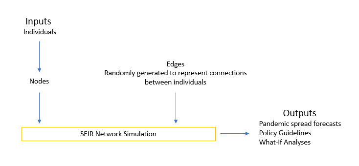
Figure 1: Current Network Simulation Setup
A major drawback of this and other network simulations is a lack of an underlying graph that accurately captures the scenario being modelled. Simulations are done on randomly generated structures, and (valuable) conclusions are drawn from these outcomes. We posit that while such analyses are useful for general guidelines, they are not effective for specific scenarios. A further shortcoming is that results and recommendations may vary widely with small changes in the underlying graph.
What’s missing?
Networks and the epidemiology of directly transmitted infectious diseases are fundamentally linked. The foundations of early epidemiological models were based on population wide random-mixing, but in practice each individual has a finite set of contacts to whom they can pass infection; the ensemble of all such contacts forms local clusters within a network, which in turn make the interactions (or connections between nodes) location-dependent.
Knowledge of the structure of the network allows models to compute the epidemic dynamics at the population scale from the individual-level behaviour of infections. Therefore, characteristics of such networks—and how these deviate from the random-mixing norm—have become important applied concerns that may enhance the understanding and prediction of epidemic patterns and intervention measures.
Uniform Manifold Approximation and Projection (UMAP)
Orthogonal to these agent-based simulations for epidemiology is the field of topological data analysis (Chazal & Michel, 2017), which infers hidden information about the structure of a complex and noisy data set using ideas from topology and geometry. TDA has been applied to the study of progression analysis of disease, signal analysis, propagation of contagions in a network, imaging and remote sensing.
One of the recent approaches for dimensionality reduction that is inspired from TDA is the Uniform Manifold Approximation and Projection (UMAP). UMAP learns the underlying topology of a point-cloud data, and tries to project it down to a lower-dimensional manifold with a near-similar topology. The results of UMAP, shown in Figure 2, demonstrate the efficacy of TDA. Taking the handwritten MNIST data set as our input, clustering using k-means forms clusters shown on the left. However, UMAP is able to perform non-linear manifold aware dimension reduction to obtain the clusters shown on the right. We anticipate similar success using location, gender and health data of individuals to use in the network simulations.
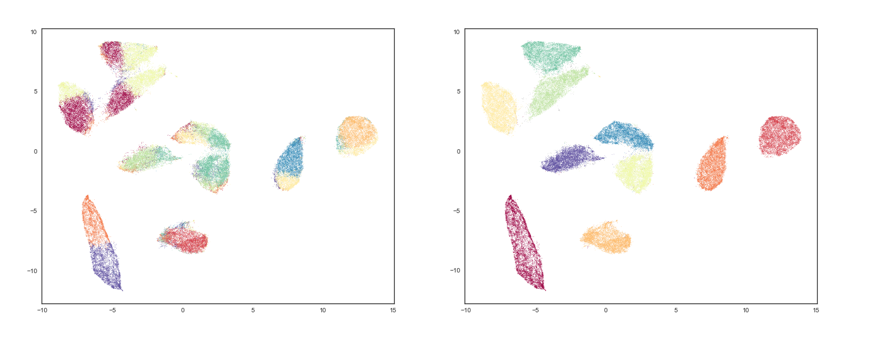
Figure 2: Clustering on MNIST using K-Means (left) and TDA/UMAP (right)
In this work, we propose to use only the first part of UMAP that employs TDA – let us call it UMAP-R. We apply UMAP-R to location data of individuals to develop networks that represent ‘ground truth’, which can then be used for agent-based simulations to analyse and predict the spread of COVID-19. Figure 3 shows how UMAP-R is integrated into the existing setup.
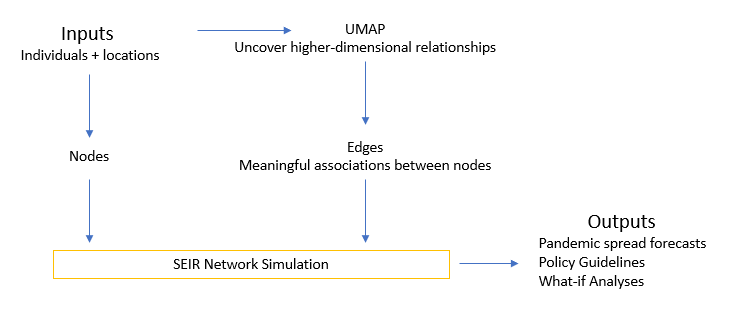
Figure 3 Using Topological Data Analysis to model the graph
How does UMAP form connections between nodes in a graph?
[The following explanation and supporting figures are presented from the excellent” UMAP Documentation by Leland McInnes]
Topological Data Analysis and Simplicial Complexes
Simplicial complexes are a means to construct topological spaces out of simple combinatorial components. This allows one to reduce the complexities of dealing with the continuous geometry of topological spaces to the task of relatively simple combinatorics and counting. This method of taming geometry and topology will be fundamental to our approach to topological data analysis in general, and dimension reduction in particular.
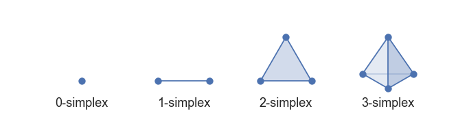
"The first step is to provide some simple combinatorial building blocks called" simplices:
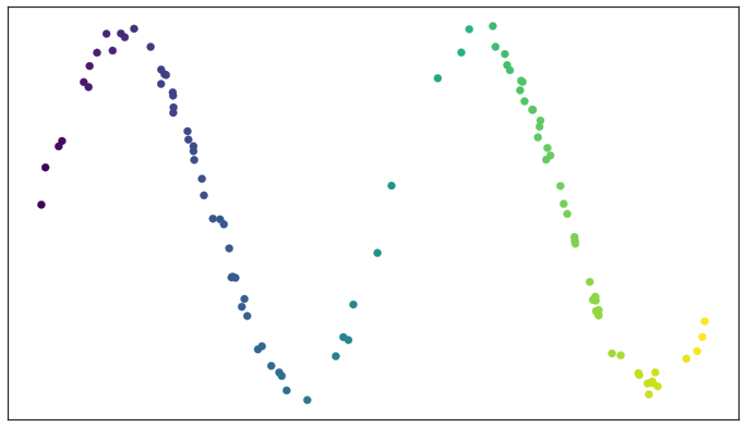
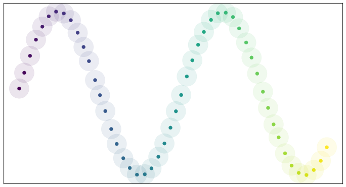
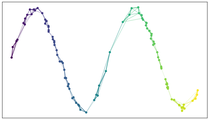
Test data set of a noisy sine wave
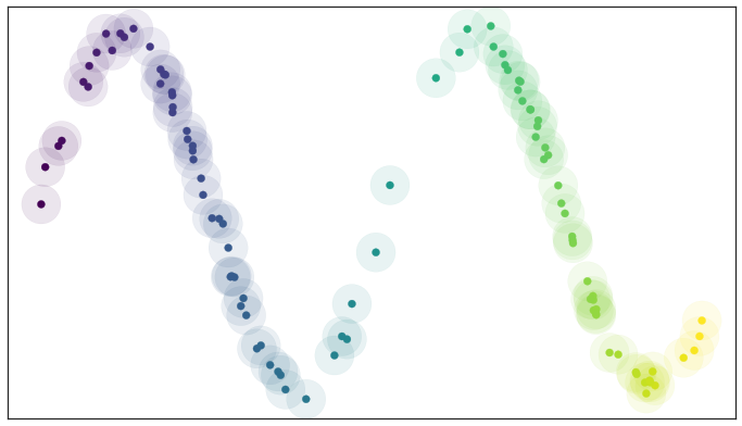
A basic open cover of the test data
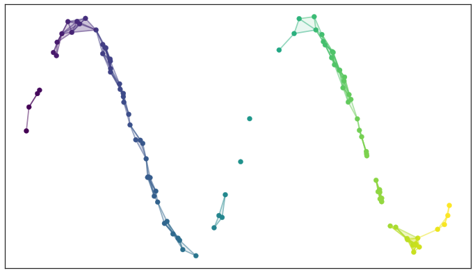
A simplicial complex built from the test data
There are two things to note here: first, the simplicial complex does a reasonable job of starting to capture the fundamental topology of the dataset; second, most of the work is really done by the 0- and 1-simplices, which are easier to deal with computationally.
Why use Topology?
The first reason is that the topological approach, while abstract, provides sound theoretical justification for what we are doing. While building a neighborhood-graph and laying it out in lower dimensional space makes heuristic sense and is computationally tractable, it doesn’t provide the same underlying motivation of capturing the underlying topological structure of the data faithfully.
The second reason is that it is this more abstract topological approach that will allow us to generalize the approach.
Adapting to Real World Data
If we consider data that is uniformly distributed, the resulting open cover looks pretty good:
Open balls over uniformly distributed data
Because the data is evenly spread we actually cover the underlying manifold and don’t end up with clumping. In other words, all this theory works well assuming that the data is uniformly distributed over the manifold. However, real-world data/spatial data under consideration isn’t that nicely behaved.
How can we resolve this? By turning the problem on its head: assume that the data is uniformly distributed on the manifold, and ask what that tells us about the manifold itself. If the data looks like it isn’t uniformly distributed that must simply be because the notion of distance is varying across the manifold.
By assuming that the data is uniformly distributed we can actually compute (an approximation of) a local notion of distance for each point by making use of a little standard Riemannian geometry. Hence, the open balls are structured such that the radius is larger in sparse regions and smaller in concentrated regions. The radius is fixed to unit distance in the riemannian terms, thus, keeping our manifold uniformly distributed. Each point is given its own unique distance function, and we can simply select balls of radius one with respect to that local distance function!
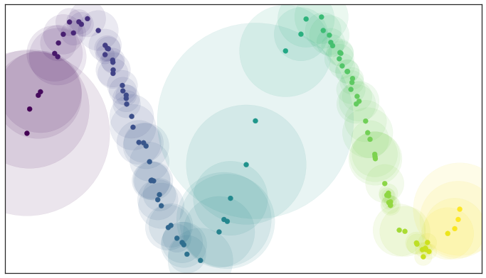
Open balls of radius one with a locally varying metric
Of course, we have traded choosing the radius of the balls for choosing a value for k. However it is often easier to pick a resolution scale in terms of number of neighbors than it is to correctly choose a distance. This is because choosing a distance is very dataset dependent: one needs to look at the distribution of distances in the dataset to even begin to select a good value. In contrast, while a k value is still dataset dependent to some degree, there are reasonable default choices, such as the 10 nearest neighbors, that should work acceptably for most datasets.
At the same time the topological interpretation of all of this gives us a more meaningful interpretation of k. The choice of k determines how locally we wish to estimate the Riemannian metric. A small choice of k means we want a very local interpretation which will more accurately capture fine detail structure and variation of the Riemannian metric. Choosing a large k means our estimates will be based on larger regions, and thus, while missing some of the fine detail structure, they will be more broadly accurate across the manifold as a whole, having more data to make the estimate with.
We also get a further benefit from this Riemannian metric based approach: we actually have a local metric space associated to each point, and can meaningfully measure distance, and thus we could weight the edges of the graph we might generate by how far apart (in terms of the local metric) the points on the edges are. In slightly more mathematical terms we can think of this as working in a fuzzy topology where being in an open set in a cover is no longer a binary yes or no, but instead a fuzzy value between zero and one. Obviously the certainty that points are in a ball of a given radius will decay as we move away from the center of the ball. We could visualize such a fuzzy cover as looking something like this:
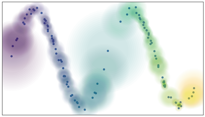
Fuzzy open balls of radius one with a locally varying metric
One of the assumptions that we need to make for riemannian geometry is that our data must be locally connected. Simply put, no point must be completely isolated from the rest of the data. To ensure this, we can implement this by simply having the fuzzy confidence decay in terms of distance beyond the first nearest neighbor. We can visualize the result as:
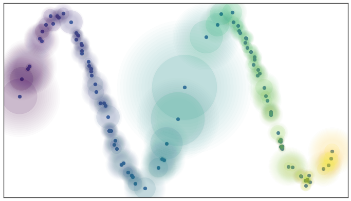
Decaying Fuzzy Confidence
OFrom a practical standpoint – in high dimensions distances tend to be larger, but also more similar to one another (the curse of dimensionality). This means that the distance to the first nearest neighbor can be quite large, but the distance to the tenth nearest neighbor can often be only slightly larger (in relative terms). The local connectivity constraint ensures that we focus on the difference in distances among nearest neighbors rather than the absolute distance (which shows little differentiation among neighbors).
Lastly, between any two points we might have up to two edges and the weights on those edges disagree with one another. Mathematically we actually have a family of fuzzy simplicial sets, and the obvious choice is to take their union – a well-defined operation.
In graph terms what we get is the following: if we want to merge together two disagreeing edges with weight a and b then we should have a single edge with combined weight a+b−a⋅b.
The way to think of this is that the weights are effectively the probabilities that an edge (1-simplex) exists. The combined weight is then the probability that at least one of the edges exists.
If we apply this process to union together all the fuzzy simplicial sets we end up with a single fuzzy simplicial complex, which we can again think of as a weighted graph.
Graph with combined edge weights
Epidemic Modeling using SEIR Compartment Model
The above obtained structure-aware graph network is fed to an SEIR Model to obtain corresponding epidemic curves.
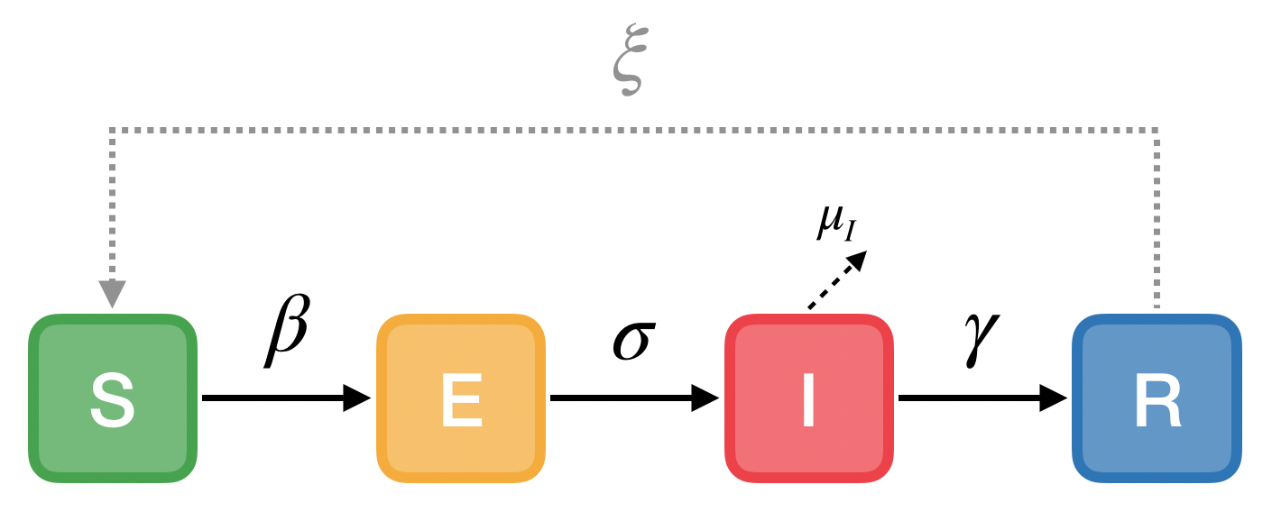
SEIR model of infectious disease
The rates of transition between the states are given by the parameters:
σ: rate of progression (inverse of incubation period)
γ: rate of recovery (inverse of infectious period)
ξ: rate of re-susceptibility (inverse of temporary immunity period; 0 if permanent immunity)
μI: rate of mortality from the disease (deaths per infectious individual per time)
Sample Output:
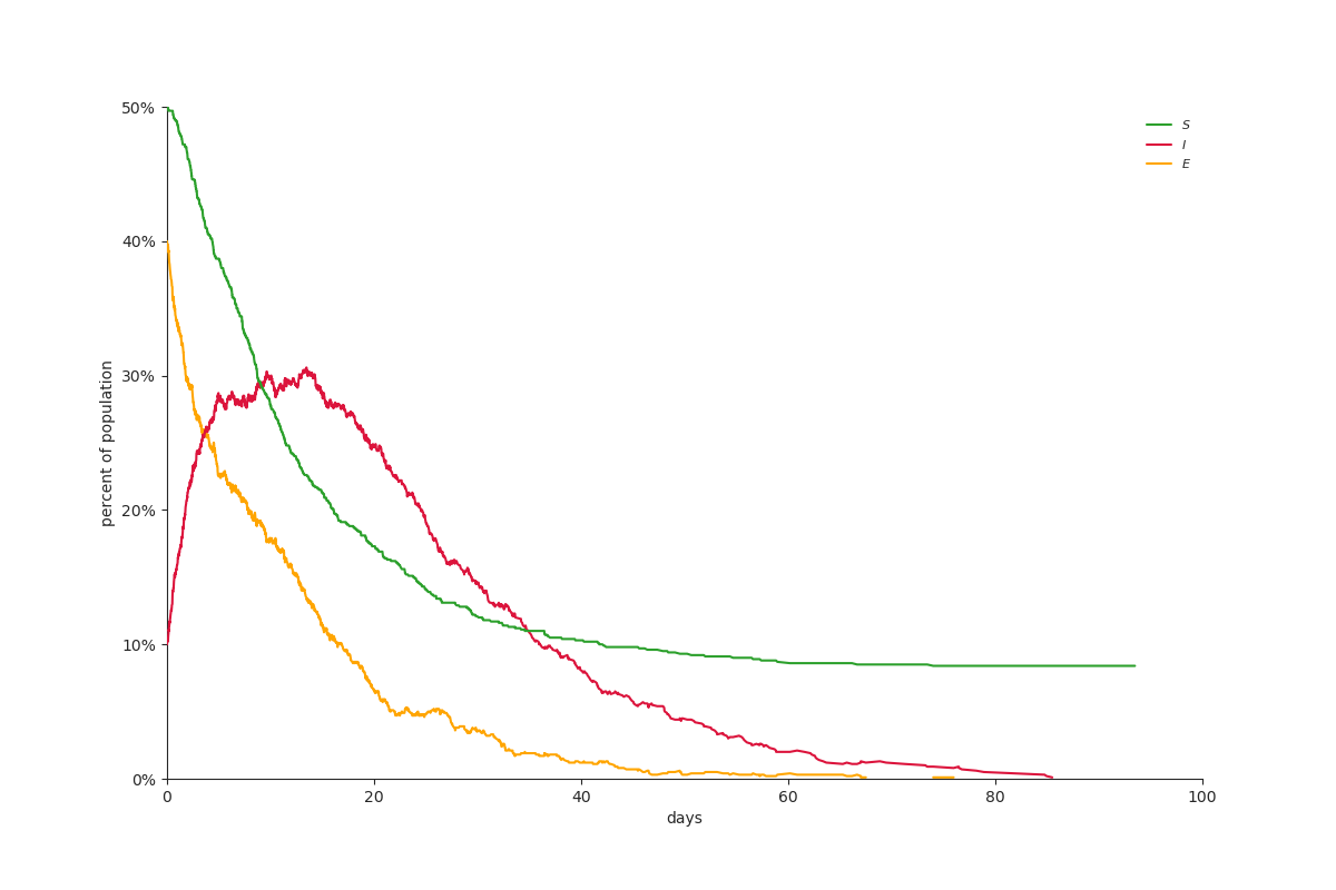
SEIR plot
[Coming Soon: Comparative analysis of epidemic curves of our TDA/UMAP based model vs models involving random connections]